← All projects

ESP32 irrigation system

V1–V3 · How it evolved

The research, tests, and engineering decisions behind each version—from the first sensor readings to independent watering control.

Follow the main story below, or expand the technical details to inspect the tests, timing logic, and supporting records.

Research

The physics behind capacitive soil sensing

I researched how electric fields, polarization, and capacitance explain the sensor’s response to moisture. This background helped me connect the voltage readings to what was happening around the probe.
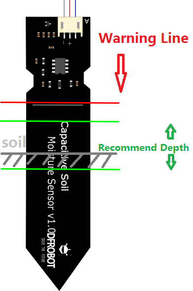
DFRobot capacitive soil sensor illustration showing the recommended insertion region below a red warning line that protects the electronics
DFRobot insertion-depth illustration, supplied as a reference. This is a similar probe, not a confirmed match to my sensor. Follow your own sensor’s markings; the lines do not show electric-field reach.

The soil becomes part of the measurement

A capacitive probe has conductive electrodes whose electric field extends beyond the board into nearby material. These curved, outward-reaching fields are called fringing fields. They let the probe respond to the soil around it instead of keeping the field entirely inside a component.

Water has a much higher permittivity than air. As water replaces air in soil pores, the material’s effective permittivity generally rises, increasing the probe’s capacitance. The sensor’s electronics turn that change into an output voltage. In my tests, wetter samples produced lower output voltages.

The electrode geometry determines how the field spreads; it is not a fixed 180-degree curve or a sharply bounded sensing distance. This explains why the material close to the probe and consistent placement matter.

Explore the electric fields, polarization & equations

1. Electric fields act on charges

Electric fields point away from positive charges and toward negative charges. The force on a charge is F = qE: a positive charge feels a force along the field, while a negative charge feels a force in the opposite direction. Like charges repel and opposite charges attract; “positive force” alone does not mean repulsion. For two point charges, the force magnitude is F = k|q₁q₂| / r².

2. The surrounding material polarizes

An applied field can slightly shift a bound electron cloud relative to its positive nucleus. This separates the centers of positive and negative charge without necessarily giving the atom a net charge. Water molecules already have positive and negative ends; an applied field tends to align these permanent dipoles.
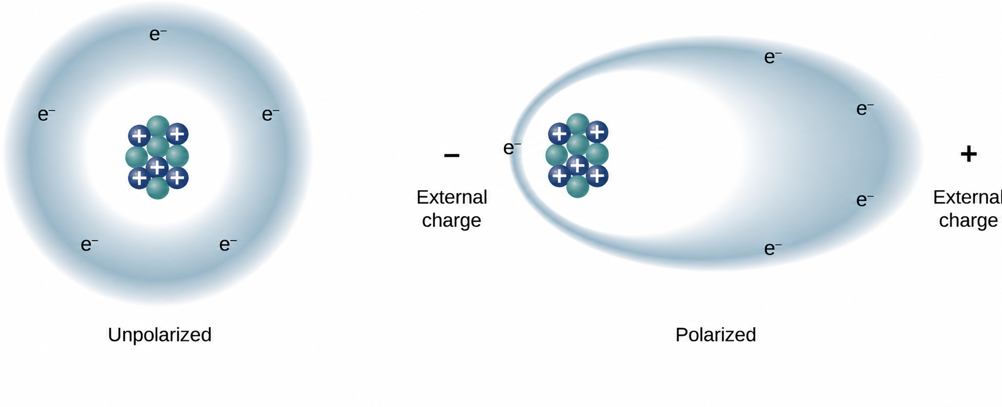
Unpolarized atom beside a polarized atom whose electron cloud shifts toward an external positive charge while its positive nucleus shifts toward an external negative charge
Induced polarization, exaggerated for illustration—not a drawing of a water molecule. Adapted from a user-supplied crop of OpenStax, University Physics Volume 2, Figure 8.19, with AI-assisted image cleanup. Access for free at OpenStax · CC BY-NC-SA 4.0.

In the simple dielectric-filled capacitor model, polarization produces bound charges whose field opposes part of the field from the plate charges. This is electric-field superposition, not destructive interference between traveling waves. Permittivity describes a material’s electrical response, including polarization; it is not itself an amount of stored energy.

3. Capacitance changes—not just voltage

Capacitance means charge stored per volt: C = Q / V. An ideal parallel-plate capacitor has C = εA / d, where ε is permittivity, A is plate area, and d is separation. Higher permittivity increases capacitance. This formula illustrates the principle; it is not an exact model of the probe’s fringing-field geometry.

For an isolated capacitor with fixed charge Q, increasing C lowers V = Q / C; the charge does not disappear. If a supply instead holds voltage constant, more charge can be stored. The relation V = Ed applies to the voltage magnitude across a uniform field along the separation—not directly to the probe’s curved, nonuniform field.

Voltage is energy per unit charge, not energy itself. A capacitor’s stored energy is U = CV² / 2 = Q² / (2C). Whether that energy increases or decreases when capacitance changes depends on whether voltage or charge is held fixed.

4. Why my board gives a lower voltage when wet

The ESP32 reads the sensor board’s processed analog output, not simply the voltage across an isolated capacitor. A change in capacitance changes the circuit’s response, which the board converts into that output. The lower reading in water is consistent with my measurements and DFRobot’s documented inverse response for a similar sensor; it cannot be derived from V = Q / C alone without knowing the circuit.

Water’s relative permittivity is roughly 80 under room-temperature, low-frequency conditions, compared with about 1 for air. Actual readings also depend on frequency, the soil mixture, and placement. The explanation does not establish a universal moisture percentage or watering threshold.

References

Finding the soil sensors’ voltage range

I tested the soil-moisture sensors in dry air and pure water to establish the approximate upper and lower voltage readings for this build. The readings varied by about ±0.02 V around these values.

Endpoint measurements, temperature checks & test limits
Observed sensor readings in the endpoint tests
Test conditionApproximate readingReference point
Dry air2.66 V ±0.02 VUpper / dry endpoint
Pure water0.80 V ±0.02 VLower / wet endpoint

I also tested the sensors in hot and cold air and observed approximately the same voltage readings in both conditions, within the variation above.

These tests established the approximate minimum and maximum of my observed voltage range: lower voltage indicated wetter conditions, while higher voltage indicated drier conditions. I used those endpoints as a reference when developing the V1 voltage bands and later V2 watering settings.

These are measurements from this project’s tests, not universal sensor limits or a direct soil-moisture percentage. The hot/cold comparison describes the conditions tested; it does not establish performance across every temperature. The watering thresholds and durations were control settings, not values determined by the endpoint measurements alone.

Choosing the watering threshold

I prepared three cups containing approximately equal amounts of spent coffee grounds, labeled dry, moist, and very moist. Initially, I added no water, three bottle-capfuls, and five bottle-capfuls respectively, mixed the wetted samples, and adjusted their water content based on my observations. The capfuls were approximate amounts, not measured volumes.

I repeatedly tested each cup, removing the sensor and cleaning off adhering grounds between insertions. The dry sample read approximately 2.3 V, the moderately moist sample around 1.8 V, and the very moist sample approximately 1.2 V. These comparisons helped me select 1.75 V as a practical watering threshold: readings above it requested watering, while readings at or below it were treated as sufficiently moist by the controller.

This was an exploratory test using qualitative moisture categories and approximate water amounts—not a calibrated measurement of soil-water content. It informed the initial control setting rather than establishing a universal threshold for every soil type. The dry coffee-ground reading is separate from the 2.66 V dry-air endpoint above.

Background research

Sensor calibration reference: DFRobot’s capacitive soil-moisture sensor calibration guide explains how dry and wet reference readings help interpret capacitive soil-moisture sensors. It also notes that insertion depth and soil packing affect the results. For this project, I selected the 1.75 V watering threshold through repeated tests with dry, moist, and very moist samples.

This reference was added while documenting the project. It covers a similar sensor, not a confirmed match to the model used here, and does not independently validate the 1.75 V setting.

Why I added a second soil sensor

Moving one sensor only a few centimeters changed its reading by approximately 0.2–0.3 V. That made a single location’s reading an uncertain basis for the watering decision. I added a second sensor and combined repeated measurements from both locations.

Two-sensor sampling method & observations
  1. Take six samples per sensor at 100 ms intervals.
  2. Calculate each sensor’s average.
  3. Average those two results into the final voltage reading.

The sampling takes approximately half a second per sensor, or about one second for both sampled sequentially. Averaging reduces dependence on a single instantaneous reading at one location. I found the combined readings more useful for the watering decision, but did not establish a formally measured accuracy improvement against a reference instrument.
Build & testing

From the first working prototype to outdoor integration testing: V1 established the core connections, V2 added Ethernet time synchronization and email monitoring, and V3 introduced independent Receiver control and the Transmitter wake-up algorithm.

Testing status: Control-system integration testing is complete; tubing tests and full-season evaluation remain. Read the project status and next-season plan →

V1 · Testing & debugging · V2 · Ethernet & email · V3 · Independent control

V1 · Testing & debugging

Version 1 established the basic connections one stage at a time: communication, low-power operation, soil sensing, valve switching, then a working two-ESP32 system. Tests 2–4 focus on the Transmitter; Test 5 focuses on the Receiver.

Original watering logic · Drier soil, longer watering

The first version explored a variable-duration concept: use the average soil-sensor voltage to choose how long to water, with longer runs for drier readings. At or below 1.75 V, watering was skipped; above that threshold, three voltage bands selected a 1-, 1.5-, or 2-hour run. We later decided the different durations were unnecessary for this garden and used two hours whenever watering was needed, while retaining the moist-soil cutoff.

Original voltage bands & duration table
Original variable-duration concept using the rounded soil voltage
Soil-voltage conditionProposed watering duration
No water needed · ≤ 1.75 VSkip watering
Water needed · > 1.75 V and < 2.00 VWater for 1 hour
Water needed · ≥ 2.00 V and < 2.25 VWater for 1.5 hours
Water needed · ≥ 2.25 VWater for 2 hours

These are the original watering-duration settings, separate from the shortened bench-test timings documented below. Exactly 1.75 V means no watering; exactly 2.00 V selects 1.5 hours, and exactly 2.25 V selects 2 hours.

In V1, opening the solenoid to water depended on the Transmitter ESP32 sending a message. Without that message, the Receiver ESP32 would not start watering. We addressed this in V3’s independent Receiver design, where the baseline and garden missing-report settings are explained.

See how V2 changed the durations →

  1. Test 1: ESP-NOW communication

    Test focus: Transmitter ESP32 + Receiver ESP32

    What is ESP-NOW? ESP-NOW is Espressif’s way of sending short wireless messages directly between compatible boards, including ESP32s. It uses the ESP32’s built-in Wi-Fi radio, but the boards do not need to connect to a Wi-Fi router or the internet to exchange messages. We chose it so our ESP32 boards could communicate directly without an extra radio module.

    How does a message reach the right board? Each board’s Wi-Fi interface has a MAC address—like a delivery address. For this setup, record each board’s Wi-Fi MAC address and configure the intended recipients in the firmware. When sending to a specific board, ESP-NOW includes that board’s address in the message header so the receiving board can identify that the message is intended for it. The MAC address is part of the header, not the whole header. The communicating boards must also use the same Wi-Fi channel.

    Espressif’s official ESP-NOW guide ↗

    How the wireless signal travels · The physics behind the radio

    I researched how wireless signals physically travel between the ESP32 boards. This is the mental picture that helped me understand it.

    Picture a bowling ball on a trampoline

    Picture a bowling ball pulling down on a trampoline. Now imagine pushing it farther down and then letting the surface rise again. The shape around the ball changes, and a ripple travels outward. The ball stays nearby, but the disturbance moves across the trampoline.

    I picture the antenna in a similar way. The ESP32’s radio circuit uses power to drive electrons back and forth. As their motion changes, they produce changing electric and magnetic fields that travel outward as a radio wave. The electrons stay in the antenna; the wave carries energy to the other board. The trampoline is just a way to visualize that traveling disturbance—radio waves do not need a surface or air to travel through.

    Think about frequency and strength, like sound

    With sound, how quickly the pressure wave repeats affects the pitch, while the size of those pressure changes affects how loud it sounds. I use that same comparison to picture a radio wave: frequency is how quickly it repeats, and amplitude is how strong it is.

    Radio can also use phase—the timing within a wave’s repeating cycle. The transmitter encodes the message using controlled patterns in the signal, called modulation. Different radio modes use different combinations of these properties; the wave’s repeating frequency is not the same as the rate at which message bits are sent.

    The other ESP32 picks up the ripple

    When the wave reaches the other antenna, its electric field pushes and pulls on electrons there, creating a tiny electrical signal. The receiving radio selects the channel, amplifies that signal, and decodes its pattern into bits.

    Those bits include the destination MAC address in the header. The receiving hardware checks that address—essentially, “Hey, is this message for me?”—and whether the frame is valid. An accepted ESP-NOW message can then reach the program, such as a soil reading sent to the Receiver. The address is checked after decoding the signal, rather than being recognized directly by an electron.

    This explains the physical radio link. ESP-NOW supplies the messaging rules on top of that link; it does not require the boards to join a router’s Wi-Fi network.

    References: OpenStax · Electromagnetic waves and antennas · NI · Radio-frequency and modulation terminology · Espressif · ESP-NOW frame format.

    Establish two-way wireless communication before adding sensors or valve control. A changing number makes each successful round trip visible in the serial monitors.

    Test setup and expected behavior
    • The Transmitter sends PAIR_REQUEST; the Receiver responds with PAIR_ACK.
    • The Transmitter sends a number. The Receiver doubles it and sends it back; the Transmitter adds one and sends it again.
    • Both serial monitors run at 115200 baud so the exchange can be followed on each board.
  2. Test 2: Sleep and wake cycles

    Test focus: Transmitter ESP32

    Check that the Transmitter can wake periodically and return to deep sleep, supporting the plan to save energy between soil readings.

    What stays on during deep sleep? The ESP32’s main processors and Wi-Fi radio power down to save energy. Its low-power RTC (real-time clock) timer keeps track of when to wake up. RTC memory also keeps the test’s wake counter, so the timer is not the only part that remains powered. Other parts of the development board can still draw power.

    What happens when it wakes? Deep-sleep wake-up restarts the program through the ESP32’s boot process, including the bootloader. Arduino then runs setup() once for that wake-up. Normally, loop() repeats after setup() finishes—but this test goes back to sleep inside setup(), so its empty loop() is not reached.

    Test setup and expected behavior
    • The test uses an approximately 10-second wake cycle and a retained wake counter to track repeated wakeups.
    • The wake counter survives deep sleep, but resets after a power loss or hard reset.
    • The README records this test as passed. The sleeping board also felt cooler than the always-on board; this was a qualitative observation, not a measured battery-life result.

    The Test 2 cycle:

    1. On startup or wake-up, setup() increases the counter stored with RTC_DATA_ATTR.
    2. It starts the Wi-Fi radio, initializes ESP-NOW, and adds the Receiver’s address again. This restores direct board-to-board messaging; it does not connect to a Wi-Fi router.
    3. It sends the wake message and waits up to 1.5 seconds for the Receiver’s reply.
    4. It sets a 10-second wake-up timer with esp_sleep_enable_timer_wakeup(), then enters deep sleep with esp_deep_sleep_start(). When the timer expires, the boot process starts again.

    The 10 seconds is the sleeping time; each full cycle also includes the time spent booting and exchanging messages. The wake counter counts wake-ups—it is separate from the RTC timer that controls the sleep interval.

    Espressif’s deep-sleep and RTC documentation ↗

  3. Test 3: One soil-moisture sensor

    Test focus: Transmitter ESP32

    Connect a real capacitive soil-moisture sensor and check that the Transmitter can turn an analog reading into a threshold-based watering decision.

    Test setup and expected behavior
    • The sensor is powered from 3V3 and GND, with its analog output connected to GPIO32 / D32.
    • On each approximately 10-second wake cycle, the Transmitter prints the raw analog reading and calculated voltage.
    • At 2.0 V or above, this early test prepares and sends TURN_ON with the reading. This checks the command path; it does not yet validate physical valve switching.
  4. Test 4: Two soil-moisture sensors

    Test focus: Transmitter ESP32

    Add a second sensor and combine both readings into one soil-moisture value, rather than making the watering decision from a single sensor.

    Test setup and expected behavior
    • The two sensors use GPIO32 and GPIO33, with power supplied from 3V3 and GND.
    • The Transmitter takes 10 samples per sensor at 10 samples per second, averages each sensor’s samples, then averages the two sensor voltages.
    • Serial output shows both sensor averages, the combined value, and the threshold comparison. A combined value of at least 1.75 V triggers the command in this test.
  5. Test 5: MOSFET and solenoid switching

    Test focus: Receiver ESP32

    Test the Receiver’s two-MOSFET switching module independently of soil sensing and radio messages, checking the control path that turns the solenoid on and off.

    Test setup and expected behavior
    • GPIO21 / D21 drives the XY MOSFET module’s signal input, with a shared ground connection.
    • A 3.3 V HIGH signal is held for 3 seconds, followed by LOW for 7 seconds. The 10-second cycle repeats continuously.
    • The expected result is solenoid activation during HIGH and deactivation during LOW. Each control-state change is printed to the serial monitor.
  6. Test 6: First integrated irrigation system

    Test focus: Transmitter ESP32 + Receiver ESP32

    Bring sensing, ESP-NOW communication, sleep cycles, and solenoid switching together. The wet/dry soil-bag desk demonstration shows the first connected system working before soldering.

    Test setup and expected behavior
    • The initial Test 6 sketch averages six readings from one sensor, compares the voltage against 1.75 V, and sends TURN_SOLENOID_ON when the threshold is exceeded. It sleeps for 7 seconds; the Receiver activates GPIO21 for 5 seconds.
    • The later Proof_Of_Work variant reads both sensors and averages their readings. Its README specifies a 15-second sleep interval and a 10-second solenoid activation, making the behavior easier to demonstrate.
    • The Live_Action variant also uses both sensors, but extends sleep to 15 minutes and solenoid activation to 2 minutes. These are separate V1 configurations, not the later daily watering schedule.

    Video 1 of 3 · Wet/dry soil-bag demonstration

    Pre-solder test: the desk setup with wet and dry soil samples, demonstrating the Transmitter ESP32 connected to the Receiver ESP32. This is the V1 integration demonstration, not the later outdoor installation.

After the initial connected prototype, testing continued with the soldered assembly and an outdoor demonstration. Continue to the integration recordings →

V2 · Ethernet & email monitoring

V1 established the sensor-to-valve connection. V2 added a third board—the Ethernet ESP32—so the system could obtain real-world time and report irrigation events without a computer connected to the serial monitor.

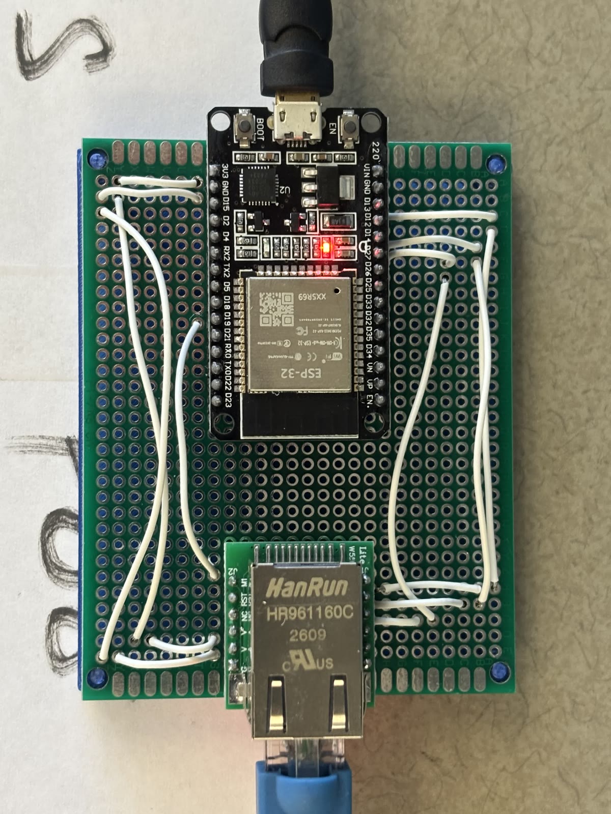
Full Ethernet ESP32 board and W5500 adapter with soldered wiring, shown sideways
Ethernet ESP32: the hand-wired board and W5500 connection.

What the Ethernet ESP32 added

  • Wired internet: a W5500 adapter connects to the network through DHCP, while ESP-NOW remains the local link between the three boards.
  • Shared time: NTP supplies Eastern local time and daylight-saving adjustments. Compact time packets synchronize the Transmitter and Receiver.
  • Email monitoring: the Receiver reports valve ON/OFF events and timestamps; the Ethernet ESP32 sends Gmail notifications through SMTP.
  • Timing-drift recovery: the archived V2 design checks reported ON times against its scheduled targets and queues a Transmitter recalibration request when the deviation exceeds ten minutes.
V2 state transitions and the move to V3

In the archived V2 firmware, the Transmitter first searches for Ethernet time, then retains a PAST flag through deep sleep to follow its recurring schedule. When its averaged voltage exceeds the threshold, it sends TURN_SOLENOID_ON; the Receiver switches the valve, acknowledges the command, and reports state changes to Ethernet. DEMO mode shortens the cycle for bench testing.

For recalibration, Ethernet sends QUEUE_RECALIBRATION to the always-awake Receiver. On the next watering command, the Receiver forwards RECALIBRATE_TIME before acknowledging it. The Transmitter resets its time-search state. A limitation was that a moist-soil wake sent no watering command, leaving a queued recalibration waiting.

V3 revised the Transmitter’s timing and made Receiver control independent →

The V2 archive contains evolving settings: the README describes 7 a.m./7 p.m. targets and a 40-minute run, while the saved final sketches use 8 a.m./8 p.m. targets and a one-hour run. The transmitter sketch uses voltage above the threshold to trigger watering, despite reversed wording in parts of the README. The email records across development include additional revisions, rather than documenting only this archived V2 protocol.

V2 watering logic · Same threshold, two-hour runs

During garden testing, we found the shorter runs were not providing enough water and decided that separate durations were unnecessary for this installation. We simplified the original variable-duration settings to two-hour runs while retaining the moist-soil cutoff, as shown below.

Garden watering bands & configurable durations
V2 garden setting · Same voltage bands, longer watering runs
Average soil-sensor voltageV2 watering duration
1.75 V or lowerNo watering
Above 1.75 V, below 2.00 V2 hours
2.00 V to below 2.25 V2 hours
2.25 V or higher2 hours

The bands remained configurable, so different durations could be restored later.

The later missing-report behavior is separate from these voltage-based duration settings. V3 explains how the Receiver gained its own watering decision and fallback →

This was a setting for this garden, not a general rule that more water is always better. The email examples across development preserve both the earlier one-hour configuration and approximately two-hour runs.

V3 · Independent control & wake-up timing

V3 focused on when the Transmitter wakes and who controls watering. The Transmitter became a scheduled soil-data source, while the Receiver could run its watering schedule even if no Transmitter message arrived. A DEMO/LIVE boolean selected short test cycles or the real daily schedule.

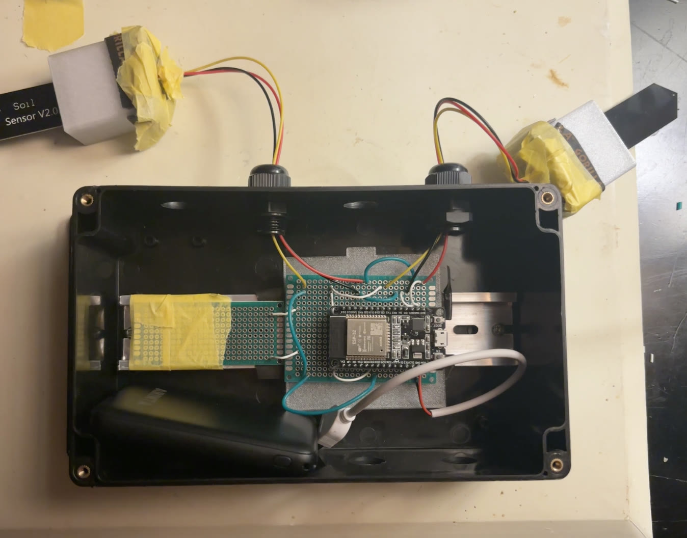
Open Transmitter enclosure containing the ESP32, soldered perfboards and battery pack, with two soil sensors connected through cable glands
Transmitter · Soil sensingTwo soil probes feed the battery-powered ESP32 inside its protective enclosure. Open full-size photo ↗
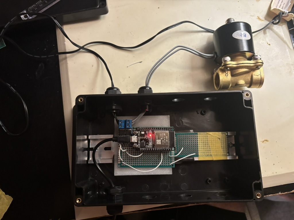
Open Receiver enclosure containing the ESP32 and switching circuit on perfboard, connected to the external brass solenoid valve
Receiver · Valve controlThe ESP32 and switching circuit connect to the external solenoid valve. Open full-size photo ↗

Naren’s staged wake-up algorithm

During early testing, we observed that long sleep intervals caused the Transmitter to wake earlier than intended. Waking every hour to request fresh time was an alternative, but we wanted to avoid that many wakeups. My mentor and supervisor, Naren Suri, developed the staged wake-up algorithm to balance extended sleep with periodic time corrections.

The scheduling logic below follows the archived V3 Transmitter firmware. On each wake, the Transmitter attempts to request fresh time from the Ethernet ESP32. During an intermediate scheduling wake, it recalculates the time remaining until 7:40 p.m. and chooses the next sleep interval. The Receiver independently owns the 8:00 p.m. watering decision.

Sleep-stage table, isRead behavior & firmware reference

Let X be the current time, Y the 7:40 p.m. target, and Z = Y − X the time remaining. If the difference is negative, add 24 hours to target the next day. At 7:41 p.m., for example, Z is 23 hours and 59 minutes.

Archived V3 Transmitter · Sleep selection when isRead is false and fresh time is available
Time remaining (Z)Sleep durationTime remaining after sleep, ideally
12 hours or moreZ − 9 hours; keep isRead = false9 hours
9 hours or more, but less than 12 hoursZ − 2 hours; keep isRead = false2 hours
More than 75 minutes, but less than 9 hoursZ − 1 hour; keep isRead = false1 hour
More than zero, up to and including 75 minutesSet persistent isRead = true, then sleep for ZTarget time
Exactly at the target (Z = 0)Take the soil reading and attempt the report immediately; do not sleep firstAlready at target

With 20 hours remaining, for example, the Transmitter sleeps for 11 hours, ideally waking with 9 hours left. It then requests fresh time and recalculates rather than assuming the sleep clock was exact. Exactly 12 hours enters the first branch; exactly 9 hours enters the second; exactly 75 minutes enters the final-sleep branch.

How the persistent isRead flag controls the next wake

The firmware declares RTC_DATA_ATTR bool isRead = false; so the flag survives deep sleep. Intermediate stages leave it false. At 75 minutes or less, the Transmitter sets it true before sleeping for the remaining interval. The 75-minute guard window avoids repeated tiny sleeps around the one-hour boundary.

On the next wake, the Transmitter attempts to get fresh Ethernet time first, then checks isRead. If true, it samples the soil and attempts to send the moisture report—even if the time request failed. It does not run the sleep-stage calculation again on that final read wake. The report contains soil status, not a command to open the valve.

After the report attempt, the firmware clears isRead = false and sleeps for one hour before starting the next scheduling cycle. On an intermediate wake with isRead = false, a failed time request instead causes a one-hour sleep before trying again. Deep-sleep retention does not mean the flag survives loss of power.

Firmware reference and timing limits

This explanation follows Transmitter-Code/transmitter_ino_code/transmitter_ino_code.ino in the supplied ESP32-V3-Code archive: calculateSecondsUntilNextSoilRead(), the scheduling branches in setup(), and performDailySoilReadAndReport(). The raw-code copy uses the same scheduling branches.

The remaining times in the table are ideal targets, not measured timing guarantees. Sleep-clock drift and the time spent waking and requesting time can affect the actual reading time. The staged algorithm periodically corrects the schedule; it does not establish zero drift.

The Receiver does not use deep sleep: its wall power supply allows it to stay awake, handle messages, and manage the valve continuously. It requests fresh Ethernet time every hour to correct its local clock; this is hourly synchronization, not an hourly wake-up cycle.

Receiver ESP32 · No longer waiting for an ON command

Initially, having the Transmitter tell the Receiver when to water seemed logical. But a depleted Transmitter battery or a missing message could prevent watering entirely. We gave the always-awake Receiver responsibility for the scheduled decision and valve timing, with three possible inputs:

  • Sufficiently moist report: skip watering.
  • Dry-soil report: use the voltage for the watering decision and email context.
  • No report: use the configured fallback rather than wait indefinitely.

The Transmitter still reports both wet and dry conditions. This prioritizes continued watering when sensing is unavailable, although fallback watering can sometimes be unnecessary. It also reduces dependence on immediate battery replacement, which requires opening the protective enclosure and potentially exposing the electronics to water. Battery maintenance is still necessary.

Missing-report settings: baseline versus final garden configuration

Missing-report settings: when no valid soil report arrived for the day, the independent Receiver’s documented baseline defaulted to one hour of watering. The final garden configuration used two hours instead. These are later independent-Receiver settings, not a fallback available in the message-triggered V1 tests. A missing report is also different from a valid moist-soil report, which skips watering.

Independence here means independence from a Transmitter trigger, not from power or initial clock synchronization. The LIVE schedule still requires the Receiver to have obtained valid time. See the recorded ON, OFF, and skipped-watering notifications →

DEMO / LIVE · Faster testing and demonstrations

The LIVE system’s 8:00 p.m. watering schedule made repeated testing impractical. A firmware boolean selects DEMO mode for a short cycle through the complete sequence: Transmitter soil readings, wireless communication, Receiver valve control, and Ethernet email notifications.

  1. The Transmitter sleeps for approximately 10 seconds, wakes, samples the soil for approximately one second, and sends its report.
  2. The Receiver operates on a 15-second cycle. A moist-soil report arriving around the 11-second point can prevent the upcoming watering activation.
  3. At the cycle’s decision point, the Receiver reports its action to the Ethernet ESP32, which prepares and sends the Gmail notification.

These test cycles do not depend on requesting the daily scheduling time. They let me demonstrate the three-board communication, observe sleep/wake transitions and valve switching, identify problems, revise the firmware, and test again without waiting until evening.

LIVE mode uses the daily sensing and watering schedule instead of this rapid test cycle.

The DEMO intervals describe my test setup, not an exact valve-open duration or a measured timing guarantee. Email arrival is not guaranteed within the 15-second cycle. DEMO/LIVE selection also appears in the V2 archive; here it supports testing V3’s independent Receiver and revised Transmitter behavior.

Ethernet ESP32 · Same core role

Ethernet retained the time and notification role introduced in V2, keeping the main timing and control changes concentrated on the Transmitter and Receiver.

Integration testing & demonstrations

The version history above explains how the firmware evolved. These recordings document the physical build after soldering and during outdoor testing; they are grouped by testing stage rather than assigned to a specific firmware version.

The V1 wet/dry soil-bag demonstration shows the initial connected prototype. The following two recordings continue that build sequence.

Video 2 of 3 · Post-solder check

A separate recording shows the setup being tested again after the connections were soldered.

Post-solder test: checking the assembled setup after soldering.

Video 3 of 3 · Garden demonstration

I presented this post-solder garden demonstration to the Baxter International Skaneateles Fall Garden Bed Community with my mentor, Naren Suri.

Garden test: the soldered irrigation setup in action outdoors, following the pre-solder demonstration and post-solder bench check.

Next: email records across development →

Email records across development

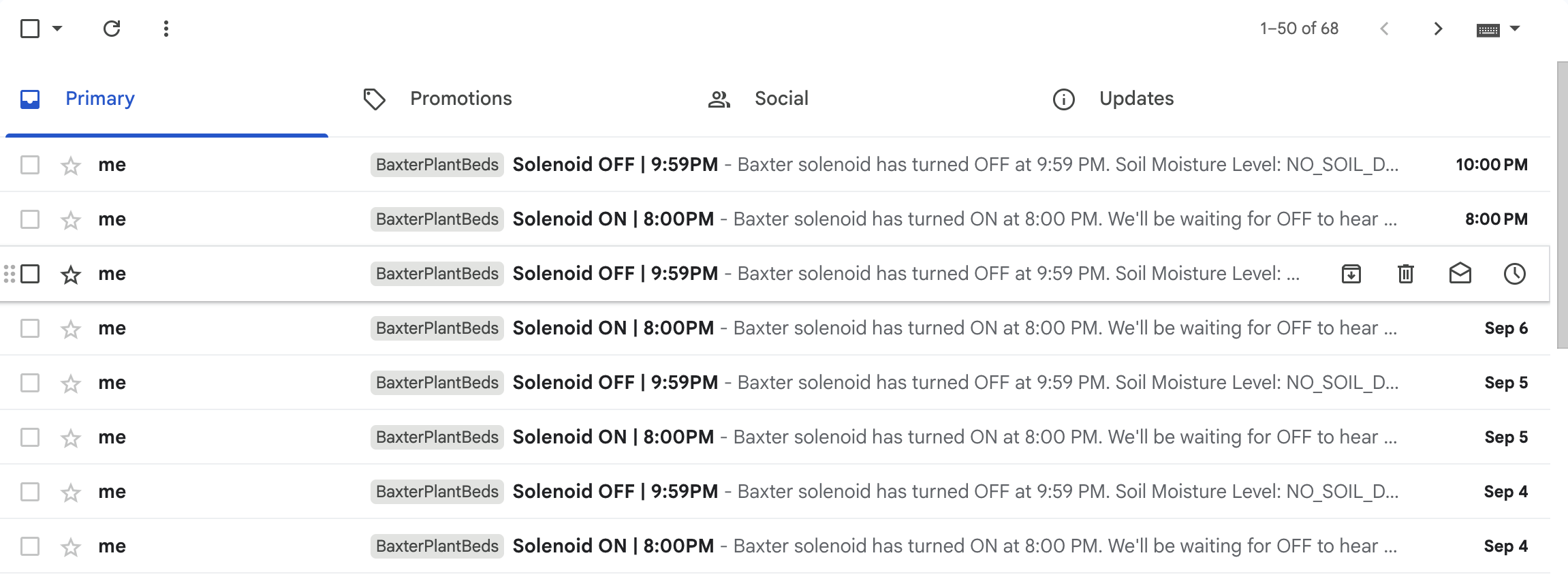
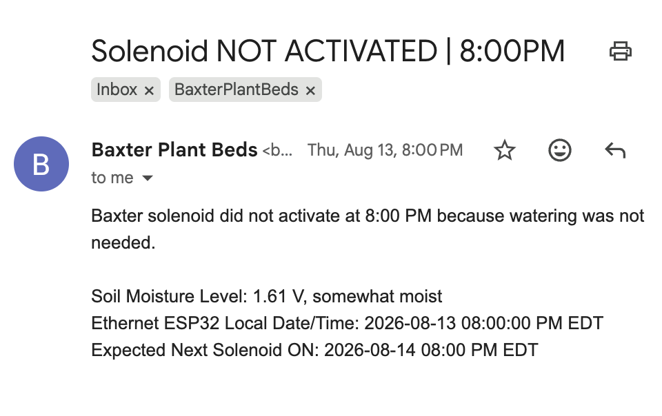
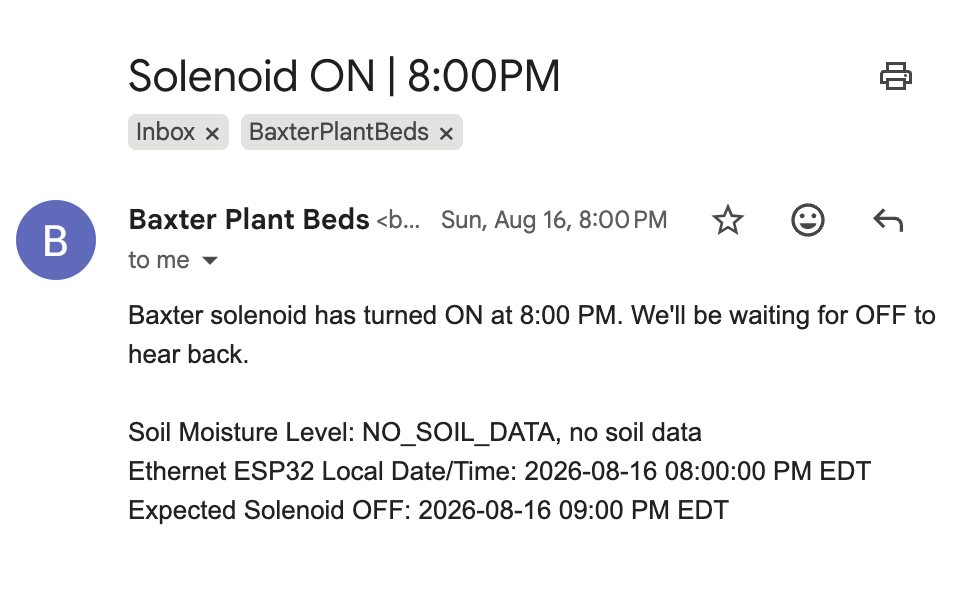
Alongside the demonstration videos, these messages show the notification capability introduced with Ethernet and its use as the garden configuration evolved. They record controller-reported events, not independently measured water flow.

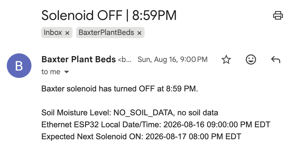
These records span different settings. Skipped-watering and missing-data notifications are not present in the archived command-only V2 protocol, so the screenshots are not presented as evidence of that version alone. The August 16 ON/OFF pair records an earlier one-hour run; the inbox history includes approximately two-hour runs. See Receiver independence and fallback settings for the control-design context.

Engineering challenges

The design evolved through decisions about testing, reliability, power management, sensing, field maintenance, and the physical irrigation layout.

Choosing the 8:00 p.m. watering schedule

We chose 8:00 p.m. to keep scheduled watering away from the brightest part of the day. At the time, we were concerned that water droplets on leaves could focus sunlight and cause scorching, even though our irrigation outlets were positioned beneath the leaves. That concern informed the schedule; it was not a mechanism we tested or demonstrated.

Horticultural clarification: ordinary watering droplets scorching leaves in sunlight is a common myth, not an established reason to avoid morning watering. Washington State University Extension generally recommends early-morning watering, notes greater evaporative losses during the day, and cautions that evening watering can encourage fungal disease when foliage stays wet. Our 8:00 p.m. setting documents this project’s choice—not a proven optimum or evidence that morning watering damages plants. Read WSU Extension’s watering guidance ↗

Related decisions explained elsewhere

The practical difficulty of outdoor firmware debugging

During final outdoor testing, I needed to verify the full chain: sensor report → Receiver action → Ethernet event → Gmail notification.

Each firmware revision required opening the protective enclosures, bringing the boards indoors to my computer, connecting them individually, uploading the revised code, and reinstalling them outside. My available laptop and network setup made indoor debugging more practical.

DEMO mode let me quickly check each revision after reinstallation. This was a hands-on cycle of updating, reinstalling, and testing the deployed hardware—not just changing code at a desk.

Changing the irrigation tubing layout

The original system used ¼-inch tubing throughout. During testing, water delivery at the outlets was weak, and some intended areas were not receiving enough water.

We changed the layout to a ½-inch main supply line feeding ¼-inch branches throughout the beds. The goal was to reduce pressure losses along the main supply path while using smaller branches to distribute water near the plants. The branches do not create additional pressure.

The observed problem and layout change are documented here; a post-change assessment of outlet flow and coverage has not yet been documented. No measured pressure or coverage improvement is claimed.

View the revised garden-bed layout →

Next: Build resources →